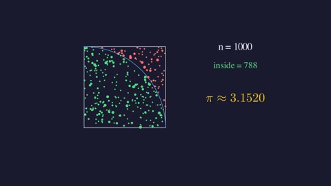
Happy Pi Day (What Casinos, Pi, and Your Retirement Have in Common)

Happy pi day. Today we are going to compute $\pi$ using nothing but random numbers, and then use the exact same technique to model your financial future.

What Monte Carlo means#

The Monte Carlo method is named after the famous casino district in Monaco. The core idea: use random sampling to estimate quantities that would be difficult to compute directly. You trade an exact calculation you cannot do for a statistical one you can, and you pay for accuracy with samples instead of cleverness.

A square, a quarter circle, and some darts#

Take a unit square, side length one. Inscribe a quarter circle in the corner, radius one. The quarter circle has area $\frac{\pi }{4}$, and the square has area $1$.

Now throw darts at the square uniformly at random. Each dart lands at some random point; some land inside the quarter circle, some outside. Because the darts are uniform, the chance any one of them lands inside is the ratio of the areas. So the fraction of darts inside approximates $\frac{\pi }{4}$:

$$\frac{\text{inside}}{\text{total}}\approx \frac{\pi }{4},\pi \approx 4·\frac{\text{inside}}{\text{total}}.$$

Multiply the observed fraction by four and you have an estimate of $\pi$. That is the whole algorithm. Generate a point, check whether it falls inside the arc, keep a running count, repeat.

Watching it converge#

Run it and watch. Every dart inside the quarter circle counts for pi; every dart outside counts against. As the count grows, the estimate stabilizes. After a hundred points it is rough. After a thousand, we are getting close to $3.14$.

The error shrinks like $\frac{1}{\sqrt{n}}$. That scaling has a sharp practical consequence: to gain one more decimal place of accuracy, you need a hundred times more samples. It is brute force. But the same brute force works in any number of dimensions, which is exactly where every clever exact method gives out.

Pause and try: how many darts for an absolute error around $0.001$?

Each dart is a coin flip that comes up "inside" with probability $p=\frac{\pi }{4}\approx 0.785$. The variance of the observed fraction after $n$ darts is $\frac{p(1-p)}{n}$, and the estimate multiplies the fraction by $4$, so its typical error is about

$$4\sqrt{\frac{p(1-p)}{n}}\approx \frac{1.6}{\sqrt{n}}.$$

Setting that to $0.001$ gives $n\approx 2.6$ million darts. Notice the shape of the answer: a thousand times better accuracy than one dart costs a million times the work, the $\frac{1}{\sqrt{n}}$ law in action.

When exact answers are out of reach#

Computing $\pi$ is a toy example; there are far better ways to get digits. Monte Carlo earns its keep when exact solutions are intractable.

Your financial future is one of those problems. The return on stocks, bonds, and real estate each year is uncertain. A single forecast of your net worth thirty years out, one number computed from average returns, is nearly meaningless: it tells you nothing about how wide the range of outcomes is or how bad the bad cases get. You need the full distribution. And no formula hands you the distribution of a thirty-year compounding process across several asset classes. So you sample it, exactly as we sampled the square.

Fitting the past#

First you need something to sample from. Aswath Damodaran at NYU Stern publishes decades of historical return data: stocks, treasury bonds, corporate bonds, real estate, all freely available online.

We fit a skew normal distribution to each asset class. Unlike a symmetric bell curve, the skew normal captures asymmetry, and the asymmetry is the point. Stock returns have a longer, fatter left side than right: crashes outrun rallies. A symmetric model quietly understates exactly the scenarios a retirement plan most needs to survive, so the shape of the left tail is not a modeling nicety. It is the risk.

Ten thousand futures#

Now run the Monte Carlo loop. Sample from the fitted distributions, one draw per asset class, and you have one possible year of returns. Chain thirty years of draws together, compounding as you go, and you have one possible financial trajectory. It is a dart, just like before: one random point from a space too complicated to integrate by hand.

Repeat ten thousand times and summarize the outcomes. Plotted together, the trajectories form a fan. The dark band covers the middle fifty percent of outcomes, the lighter bands cover ninety percent, and the median line runs through the center. Instead of one fragile forecast, you can read off questions that actually matter. What does the typical path look like? How wide is the spread by year thirty? Where do the unlucky ten percent of futures end up?

This is how professionals model long-term financial plans. The fan chart is to the retirement problem what the converging counter was to $\pi$: the moment where accumulated randomness resolves into a stable, usable answer.

One method, two payoffs#

Look at how little changed between the two halves. For $\pi$, the sampling distribution was uniform points in a square and the summary was a single ratio. For the portfolio, the sampling distribution was skew normals fitted to a century of market data and the summary was a fan of percentiles. The method in between is identical: draw random samples, push each one through the question you care about, and let the aggregate approximate what you could not compute directly.

That is the Monte Carlo method, from computing digits of $\pi$ to stress-testing a retirement portfolio. Happy pi day.

If you remember three things#

1. Monte Carlo estimates hard quantities by random sampling: the fraction of uniform darts inside the quarter circle approximates $\frac{\pi }{4}$, so four times the fraction approximates $\pi$.
2. The error shrinks like $\frac{1}{\sqrt{n}}$, so each extra decimal place costs a hundred times more samples, but the method keeps working where exact answers are intractable, including high dimensions.
3. Your financial future is a sampling problem: fit skew normal distributions to historical returns, respect the asymmetry, chain thirty years of draws, and read the fan chart, not a single forecast.